All published articles of this journal are available on ScienceDirect.

Gaussian Process Regression with Bayesian Optimisation and Uncertainty Propagation for Predicting the Fundamental Period of Masonry-infilled RC Frames

Abstract
Introduction/Objective
Reinforced Concrete (RC) frames with masonry infills represent a widely adopted structural typology in Algeria. The present study aims to predict the fundamental period of this type of structure using various machine learning algorithms.
Methods
Several machine learning models, including Gaussian Process Regression (GPR) applied for the first time to this problem, are employed to assess their performance in predicting the fundamental period of masonry-infilled reinforced concrete frames, using statistical metrics such as the coefficient of determination R2 and the Root Mean Square Error (RMSE). An uncertainty propagation analysis is subsequently conducted using the Gaussian Process Regression (GPR) model to evaluate the sources of uncertainty associated with the prediction of the fundamental period of structures.
Results
The results indicate that the GPR model achieves a coefficient of determination R2 = 0.9999 on the test data, outperforming all models previously proposed in the literature. The uncertainty analysis reveals that model-related uncertainty accounts for 7.8% of the total uncertainty, whilst input data uncertainty accounts for 92.2%.
Discussion
This study highlights the relevance of using GPR models to predict the fundamental period of reinforced concrete frames. It also addresses one of the key limitations of purely data-driven models and demonstrates the benefits of resorting to physics-informed machine learning models.
Conclusion
This study demonstrates the superiority of the GPR model over other machine learning models, whilst also outperforming the models previously proposed in the literature. An analysis of the influence of the input variables reveals that their relationships are predominantly non-linear.
1. INTRODUCTION
The typology of Reinforced Concrete (RC) frames is widespread worldwide, and Algeria is no exception. Over time, this structural form has gained prominence, particularly after the country’s independence in 1962. Past earthquakes, such as the El Asnam event in 1980, caused significant damage and collapse in this type of structure [1]. During the Boumerdes earthquake in 2003, post-seismic reports indicated that this typology accounted for approximately 90% of the damaged buildings in the affected areas. Consequently, authorities decided to restrict the slenderness of such structures according to a defined seismic zoning scheme [2]. The new RPA 2024 code introduced only minor updates, mainly by revising the slenderness limits based on the updated seismic zoning [3]. Infilled RC frame structures exhibit complex behaviour due to the interaction between two elements with contrasting mechanical properties: on the one hand, the RC frame is relatively flexible yet ductile; on the other hand, the masonry infill wall is characterised by high stiffness but pronounced brittleness. The introduction of masonry infills within the frame, therefore, profoundly alters the global structural response, enhancing both stiffness and load-bearing capacity [4, 5]. Beyond these static effects, the interaction also influences the dynamic behaviour. Indeed, numerous studies have demonstrated that the presence of infill walls leads to a significant reduction in the fundamental period of RC frames [6, 7]. In certain configurations, this reduction in period may increase the risk of resonance. As a result, a structure initially considered flexible may, once stiffened by infills and founded on stiff soil, experience amplified displacements that can heighten the probability of structural collapse.
The fundamental period of Reinforced Concrete (RC) structures is a key parameter in the design and analysis of frame systems. To estimate this period, numerous empirical models have been developed and published in the literature. Kaushik et al. (2006) [8] provided a comprehensive review of the main available formulations, highlighting that several early seismic design codes-expressed the fundamental period as a function of the building height (H) and, in some cases, the base dimension (d). However, most of these models rely on a single variable—most commonly the building height (H). This simplified approach has a significant limitation, as it neglects the influence of other parameters that may affect the variation of the fundamental period. A comparative overview of some of these empirical models is presented in Table 1.
| Reference | Formula | Comment |
|---|---|---|
| Chopra & Goel (2000) [9] | FP = 0.067 H0.9 | |
| Crowley & Pinho (2004) [10] | FP = 0.1 H | H in feet |
| Crowley & Pinho (2006) [11] | FP = 0.055 H | H in feet |
| Goel & Chopra (1997) [12] | FP = 0.053 H0.9 | |
| Guler et al. (2008) [13] | FP = 0.026 H0.9 | |
| Hong & Hwang (2000) [14] | FP = 0.0294 H0.804 | |
| RPA 2024 [3] | FP = CTH0.75 | CT = 0.075 structure without infill CT = 0.05 structure with infill |
| Verdame et al. (2010) [15] | FP = 0.135 H0.67 |
The introduction of Machine Learning (ML) methods has experienced remarkable growth in recent years [16-18], particularly in the field of earthquake engineering (Hu et al. 2025) [19]. This trend has led to an increasing number of studies aimed at assessing the effectiveness of various ML algorithms for predicting structural parameters. Among these, the fundamental period of Reinforced Concrete (RC) frames has received particular attention. The prediction of the fundamental period of RC frames infilled with masonry has gained growing interest over the past decades due to the limitations of the empirical formulas provided by seismic design codes.
The application of ML techniques has enabled the development of highly efficient predictive models. The pioneering work in this domain was conducted by Asteris et al. (2016) [7], who used a database of 1,281 masonry-infilled RC frames to train Artificial Neural Networks (ANNs), demonstrating performance significantly superior to that of traditional empirical models. Subsequently, Asteris and Nikoo (2019) [20] employed the “FP4026 Research Database” (Asteris 2016) [21] to develop ANN models optimised using a bee colony algorithm, achieving very high accuracy with R2 = 0.999. Bernardo et al. (2024) [22] generated a synthetic database of 18,000 structures and proposed two predictive models—one based on simple regression and the other on Bayesian inference—taking into account several influencing parameters.
The “FP4026 Research Database” Asteris (2016) [21] has served as a foundation for numerous comparative studies, among which Vijayan et al. (2024) [23] evaluated various algorithms—including linear regression, SVR, random forests, and ensemble learning—while Karampinis et al. (2024) [24] achieved excellent performance using Gradient Boosting (R2 = 0.993), complemented by SHAP analysis to derive interpretable empirical formulas. Shan Lin et al. (2025) [25] introduced the Kolmogorov–Arnold Network (KAN), which outperformed models such as SVR, XGBoost, CatBoost, RFR, and traditional neural networks.
Đorđević & Marinković (2024) [26] differentiated between bare and masonry-infilled frames, developing ANNs optimised through Bayesian regularisation and refined using multi-objective genetic algorithms. Other studies have confirmed the superiority of boosting-based algorithms: Yahiaoui et al. (2023) [27] identified LightGBM as the most effective and subsequently proposed an analytical formula using MARS. In a later study, Yahiaoui et al. (2025) [28] demonstrated the superiority of XGBoost over DNN and RFR, analysing the influence of the training/testing ratio. Rahman et al. (2024) [29] also confirmed the efficiency of LightGBM among seven tested algorithms, particularly in terms of computational efficiency. Dauji et al. (2024) [30] highlighted the relevance of Decision Tree Regression (DTR).
More recently, approaches integrating model interpretability have gained prominence. Thisovithan et al. (2023) [31] and Latif et al. (2022) [32] employed tools such as PDP, ICE, SHAP, and LIME, while Inqiad et al. (2024) [33] demonstrated the robustness of XGBoost compared to other evolutionary algorithms, including MEP and GEP. Deep Neural Networks (DNNs) represent another promising research direction. Bioud et al. (2023) [34] applied this approach to the FP4026 database and developed a dedicated predictive software tool for practitioners.
In parallel, several studies have relied on databases generated from 3D simulations. Ruggieri et al. (2022) [35] conducted 384 simulations to derive two distinct analytical equations depending on the presence or absence of infill, incorporating parameters often neglected—such as the mass of intermediate floors. Similarly, Kumar et al. (2025) [36] developed a database of 162 simulated frames and tested multiple algorithms (SVR, RFR, ANN, GBTR), confirming the effectiveness of ML- based approaches.
2. ORIGINALITY OF THE STUDY
While the individual techniques employed in this study are well established, their combined application and methodological integration in the context of predicting the fundamental period of infilled reinforced concrete frames constitute a novel contribution.
A first key contribution lies in the explicit introduction of interaction variables, enabling the modelling framework to capture coupled relationships between structural parameters that are not represented by the original input features. This enhances both predictive performance and physical interpretability. In addition, this study provides one of the first systematic investigations of Gaussian Process Regression (GPR) models for this specific problem, including a comparative analysis of different kernel functions, thus providing insights into how kernel choice influences the representation of structural nonlinearities. A further contribution is the integration of Bayesian optimisation into a cross-validation framework, ensuring robust and unbiased hyperparameter tuning across multiple data partitioning scenarios.
Beyond predictive accuracy, particular emphasis is placed on uncertainty quantification. A global uncertainty propagation analysis is conducted using Monte Carlo simulation in combination with the probabilistic nature of GPR, enabling the joint assessment of prediction variability and reliability, while explicitly distinguishing between input-induced and model-related uncertainty contributions.
Building on this, the combined use of SHAP-based sensitivity analysis and uncertainty propagation provides a complementary framework for model interpretability, allowing the identification of key variables while simultaneously evaluating prediction confidence. It should be noted, however, that SHAP-based interpretations remain model-dependent and reflect learned relationships rather than strict causal effects.
3. METHODOLOGY
The methodological approach adopted in the present research can be decomposed into five distinct stages, as summarised in Fig. (1).
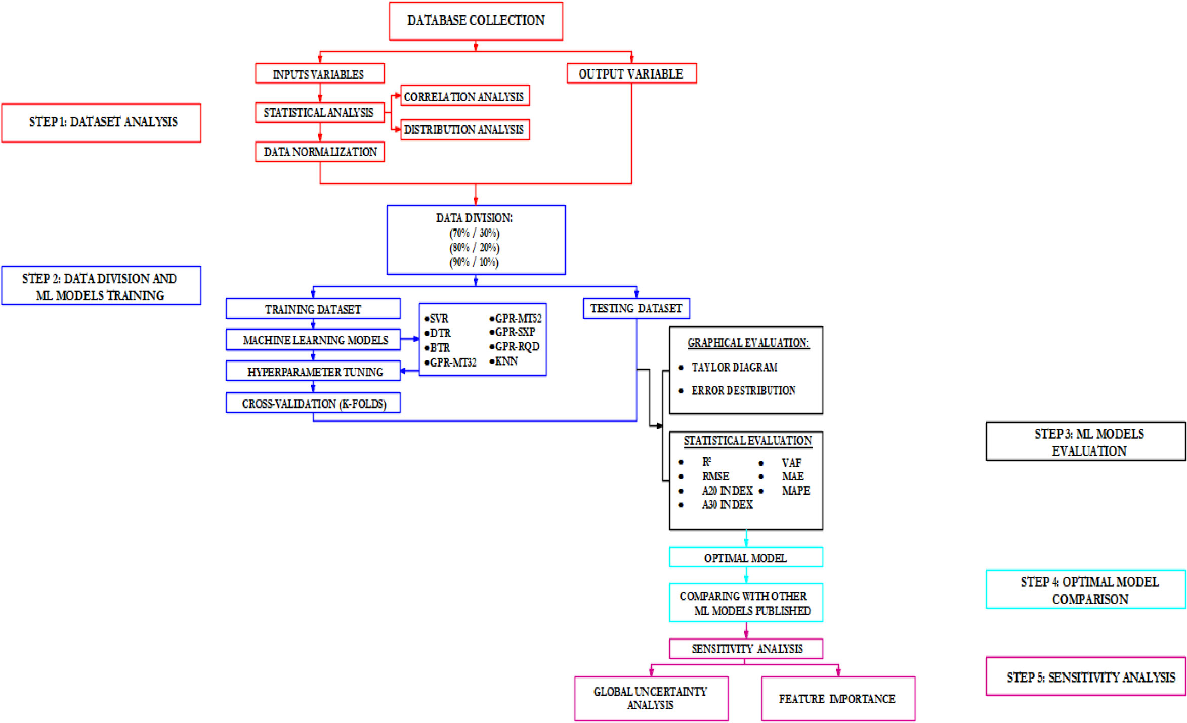
Overview of the methodology adopted in this study.
Step 1: Importation of the database and execution of a preliminary statistical analysis, including the examination of variable distributions and the assessment of correlations through a heatmap.
Step 2: The dataset was partitioned into independent training and testing subsets following an 80/20 ratio; additional split ratios were also investigated to assess their influence on model performance. All model development steps were conducted exclusively on the training set, and the test set was strictly reserved for final evaluation, ensuring clear separation between phases and preventing any data leakage. All input variables were standardised prior to training, and this preprocessing procedure was consistently applied across all models.
A ten-fold cross-validation procedure was applied within the training data to evaluate model performance during the optimisation process. Bayesian optimisation was employed for hyperparameter tuning, with candidate configurations assessed through this cross-validation scheme. The models were subsequently trained using various machine learning algorithms. In addition to Gaussian Process Regression (GPR), the following comparative algorithms were considered:
- Decision Tree Regression (DTR)
- Support Vector Regression (SVR)
- Bagging Tree Regression (BTR)
- k-Nearest Neighbours (KNN)
Step 3: Comparison of the performance of the Machine Learning (ML) models using statistical indicators such as the coefficient of determination (R2), Root Mean Square Error (RMSE), Mean Absolute Percentage Error (MAPE), Mean Absolute Error (MAE), Variance Accounted For (VAF), and the A20 and A30 indices. Graphical tools, including the Taylor diagram and error distribution plots, were also employed to complement the quantitative evaluation.
Step 4: Comparison of the obtained models with previously published ML models reported in the scientific literature.
Step 5: Sensitivity analysis using the optimal model, based on the evaluation of input variable importance through SHAP (SHapley Additive exPlanations), complemented by a global uncertainty propagation analysis.
The present research focuses on comparing the performance of various Machine Learning (ML) models for predicting the fundamental period of Reinforced Concrete (RC) frames infilled with masonry, using two complementary evaluation approaches.
The first approach is based on the assessment of statistical indicators defined by Eqs. (1–7). The coefficient of determination (R2) represents the proportion of the total variance explained by the model, while the Root Mean Square Error (RMSE) quantifies the average deviation between observed and predicted values, giving greater weight to large errors. The Mean Absolute Percentage Error (MAPE) measures the average of the absolute relative errors, and the Mean Absolute Error (MAE) corresponds to the average of the absolute residuals. The Variance Accounted For (VAF) expresses the proportion of the variance in the observed data reproduced by the model. The A20 and A30 indices represent the percentage of predictions whose relative errors are within ± 20% and ± 30%, respectively, of the observed values.
The second approach relies on graphical evaluation using complementary visual tools. This includes the error distribution plot, which helps identify potential trends or biases in the residuals, and the Taylor diagram, which provides a visual synthesis of model performance by comparing them based on three key metrics: the correlation coefficient between observed and predicted values, the standard deviation—used to assess the model’s ability to reproduce the variability of the observed data—and the centred root mean square error, which evaluates the model’s ability to replicate the pattern of the target variable after removing the mean bias.
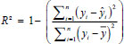
y: observed value and ŷ predicted value
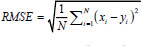
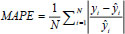
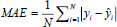
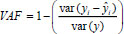
var: Variance

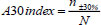
4. STATISTICAL ANALYSIS OF THE DATASET
The dataset used in this study is the Asteris [21] Database, which compiles the results of 4026 simulations on the fundamental period of Reinforced Concrete (RC) frames infilled with masonry. The output variable considered is the fundamental period of the structure (FP), while five input variables were selected: the number of storeys (STN), the number of bays (SPN), the bay length (SPL), the percentage of openings in the infill wall (OPP), and the infill wall stiffness (IFS). The IFS values were provided in the dataset in a scaled form (×105 kN/m) and were used as such in this study.
In contrast to previous studies, this research explicitly includes interaction variables to analyse their influence on the fundamental period of masonry-infilled RC frames. These interaction terms were generated using the x2fx function in MATLAB, considering pairwise combinations between the original input variables. All features were subsequently normalised to the range [0.1, 0.9] using a min–max scaling transformation prior to model training.
In total, fifteen input variables were considered. Figure 2 illustrates the statistical distribution of the data using histograms combined with Kernel Density Estimation (KDE), highlighting the range, variability, and shape of both input and output variables. Vertical lines indicate the mean and median values for each variable. A detailed description of all input and output features is provided in Table 2. Additionally, a statistical summary is presented in Table 3, providing the main indicators of central tendency, dispersion, and distribution shape.
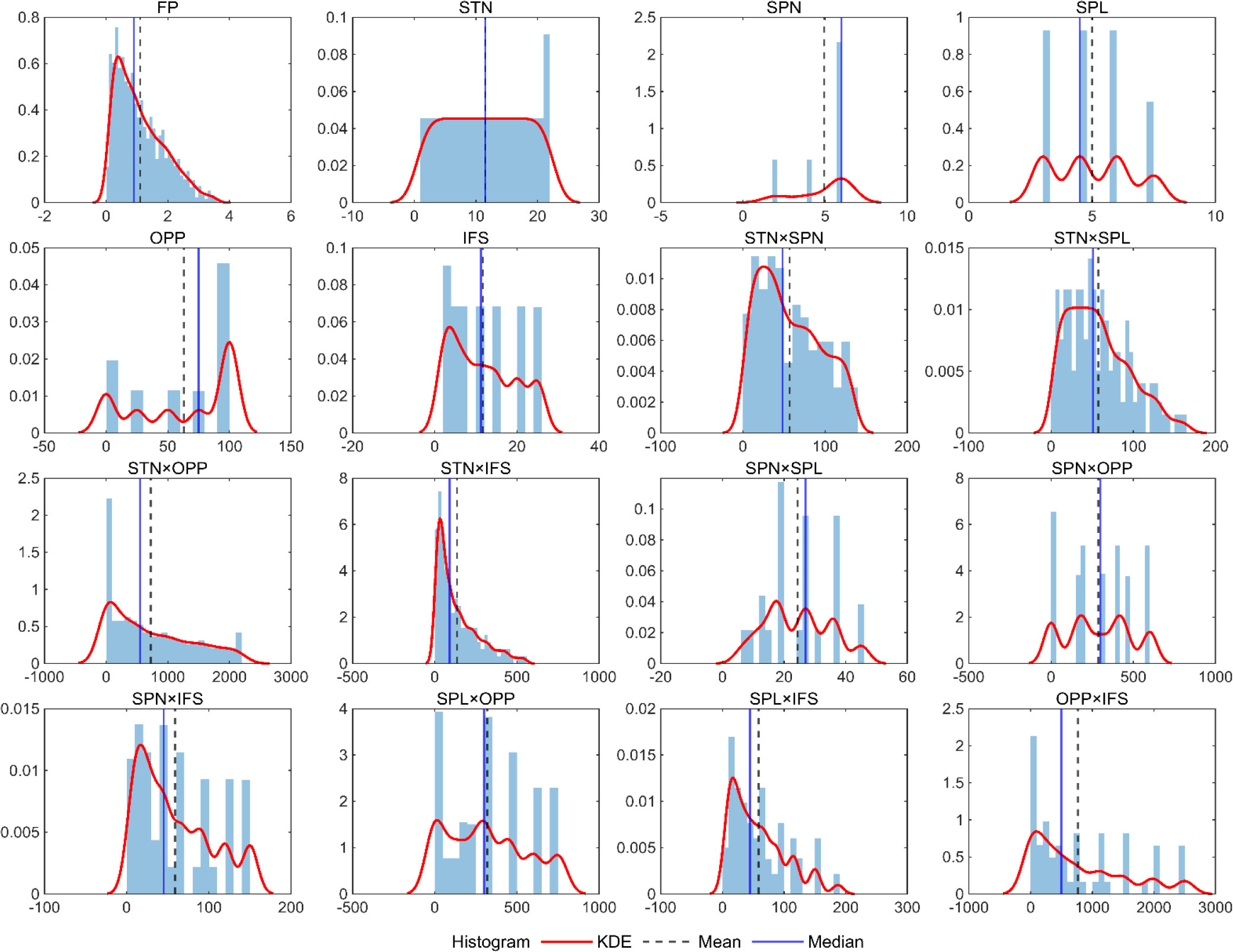
Distribution of input variables and the fundamental period (output variable).
| Features | Unit | Description |
|---|---|---|
| FP | s | Fundamental period of the structure |
| STN | - | Number of storeys |
| SPN | - | Number of bays |
| SPL | m | Bay length |
| OPP | % | Opening percentage in the infill wall |
| IFS | (kN/m) | Infill wall stiffness (scaled ×105) |
| STN*SPN | - | Interaction between the number of storeys and the number of bays |
| STN*SPL | - | Interaction between the number of storeys and the bay length |
| STN*OPP | - | Combined effect of storeys and opening percentage |
| STN*IFS | - | Combined effect of storeys and infill stiffness |
| SPN*SPL | - | Interaction between the number of bays and bay length |
| SPN*OPP | - | Combined effect of bays and opening percentage |
| SPN*IFS | - | Combined effect of bays and infill stiffness |
| SPL*OPP | - | Combined effect of span length and opening percentage |
| SPL*IFS | - | Combined effect of span length and infill stiffness |
| OPP*IFS | - | Combined effect of openings and infill stiffness |
| Parameter | Min | Max | Mean | Median | SD | Cov (%) | Skew | Kurtosis |
|---|---|---|---|---|---|---|---|---|
| FP (s) | 0.040 | 3.566 | 1.105 | 0.91 | 0.785 | 71.057 | 0.822 | -0.060 |
| STN | 1.00 | 22.0 | 11.500 | 11.50 | 6.345 | 55.175 | 0.00 | -1.205 |
| SPN | 2.00 | 6.0 | 4.951 | 6.0 | 1.548 | 31.273 | -1.050 | -0.529 |
| SPL (m) | 3.00 | 7.5 | 4.992 | 4.50 | 1.577 | 31.600 | 0.162 | -1.194 |
| OPP (%) | 0.00 | 100.0 | 63.084 | 75.0 | 40.140 | 63.630 | -0.506 | -1.376 |
| IFS (kN/m) | 2.250 | 25.0 | 11.762 | 11.25 | 7.787 | 66.204 | 0.376 | -1.170 |
| STN*SPN | 2.00 | 132.0 | 56.934 | 48.0 | 37.421 | 65.726 | 0.413 | -0.992 |
| STN*SPL | 3.00 | 165.0 | 57.406 | 51.0 | 37.847 | 65.930 | 0.671 | -0.223 |
| STN*OPP | 0.00 | 2200 | 725.59 | 550.0 | 662.084 | 91.248 | 0.645 | -0.774 |
| STN*IFS | 2.25 | 550.0 | 135.314 | 90.0 | 126.714 | 93.645 | 1.231 | 0.815 |
| SPN*SPL | 6.00 | 45.0 | 24.443 | 27.0 | 10.630 | 43.489 | 0.223 | -0.843 |
| SPN*OPP | 0.00 | 600.0 | 286.699 | 300.0 | 198.757 | 69.326 | 0.050 | -1.104 |
| SPN*IFS | 4.50 | 150.0 | 59.062 | 45.0 | 44.850 | 75.937 | 0.683 | -0.710 |
| SPL*OPP | 0.00 | 750.0 | 318.349 | 300.0 | 244.743 | 76.879 | 0.306 | -1.036 |
| SPL*IFS | 6.75 | 187.5 | 58.634 | 45.0 | 44.691 | 76.221 | 0.941 | 0.181 |
| OPP*IFS | 0.00 | 2500.0 | 769.278 | 500.0 | 755.035 | 98.149 | 0.901 | -0.287 |
From Table 3, it can be observed that the output variable, FP, exhibits a right-skewed distribution, characterised by a median lower than the mean and a very high variability, with a coefficient of variation exceeding 70%. The shape indicators confirm this positive skewness (skew > 0) and a slightly flattened distribution (kurtosis close to 0), indicating a low concentration of extreme values. Regarding the five input variables, the statistical analysis reveals balanced yet heterogeneous data, marked by considerable variability. The number of storeys (STN) shows a symmetric distribution centred around the mean, with moderate dispersion. The variables SPN and SPL display relatively homogeneous distributions (Cov ≈ 31%), although SPL is more tightly centred around the mean than SPN. The variables OPP and IFS exhibit highly dispersed distributions (Cov > 63%), with positive skewness for IFS and negative skewness for OPP. The interaction variables amplify overall data variability, with some showing coefficients of variation reaching up to 98% (OPP*IFS), while the interaction variable (SPN*SPL) presents more moderate dispersion (Cov = 43%). All interaction variables display positive skewness (mean > median). Some variables exhibit leptokurtic distributions (kurtosis > 0), whereas others are platykurtic (kurtosis < 0), confirming a broad representation of geometric plan combinations.
Figure 3 highlights, among the main variables, a strong positive linear correlation between the target variable FP (fundamental period) and the input variable STN (number of storeys), suggesting a significant linear influence of building height on the dynamic response. A moderate positive correlation is also observed between FP and the percentage of openings (OPP), indicating that an increase in the opening ratio tends to increase the fundamental period. In contrast, the very weak correlation between FP and the infill wall stiffness IFS suggests that wall stiffness, when considered in isolation, exerts only a limited linear effect on the frame period.
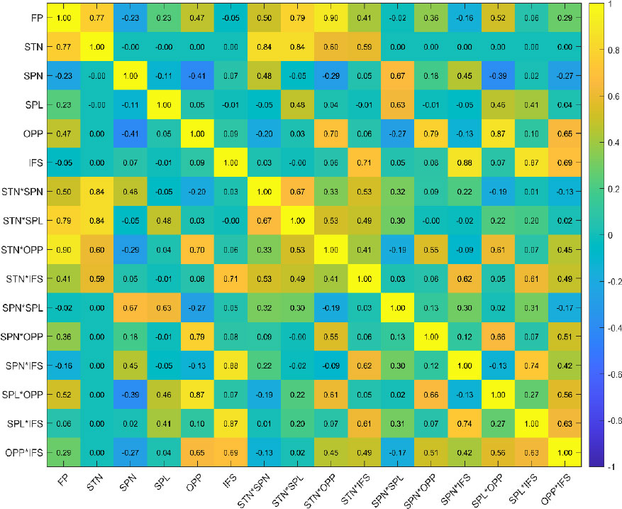
Correlation matrix between input variables and the output variable.
The geometric parameters related to the frame bays (SPN and SPL) show weak correlations (R = –0.23 and R = 0.23), reflecting a secondary influence on the fundamental period. The interaction variable STN*OPP exhibits the strongest correlation with FP (R = 0.90), emphasising the importance of incorporating the combined effects of height and opening percentage in the modelling process. Finally, correlations among the five basic input variables remain low, the most notable being between OPP and SPN (R = 0.47), confirming the weak interdependence among the input parameters. It should be noted, however, that the Pearson correlation coefficient only captures linear relationships and may not fully reflect potential nonlinear or higher-order interaction effects that could nonetheless contribute to model performance.
5. MACHINE LEARNING ALGORITHMS
Several machine learning algorithms were considered in this study, including K-Nearest Neighbours (KNN), Support Vector Regression (SVR), Decision Tree Regression (DTR), Bagging Tree Regression (BTR), and Gaussian Process Regression (GPR). These methods were implemented according to their standard formulations as widely described in the literature [37–39, 40–44].
KNN is a non-parametric method based on distance metrics, commonly used for regression and classification tasks [37–39]. SVR, originally developed by Vapnik and Lerner [45], relies on the ε-insensitive loss function to achieve robust regression performance [46]. Decision tree-based approaches, including DTR and ensemble methods such as Bagging, have been widely applied for modelling nonlinear relationships [40–44].
Particular attention was given to GPR due to its probabilistic and nonparametric nature, allowing both accurate predictions and uncertainty quantification [47–49]. In this study, the GPR model implemented in MATLAB was used with a constant basis function and four kernel functions: Matérn 3/2 (GPR-MT32), Matérn 5/2 (GPR-MT52), Squared Exponential (GPR-SXP), and Rational Quadratic (GPR-RQD).
5.1. Hyperparameter Tuning and Cross Validation
Hyperparameter optimisation was performed using Bayesian optimisation, a sequential global optimisation approach particularly suitable for computationally expensive and non-convex objective functions [48, 50]. Compared to grid search or random search, this method provides improved efficiency in exploring the hyperparameter space [29]. The “expected-improvement-plus” acquisition function was employed, with 30 evaluations performed for each model, as convergence was reached and additional evaluations did not lead to significant performance improvements. In addition, a 10-fold cross-validation strategy was applied to ensure robust model evaluation and to reduce the risk of overfitting [51]. Table 4 presents the optimised hyperparameters, the range of values tested, and their corresponding optimal values [48].
| Model | Hyperparameters | Tested values | Optimal value |
|---|---|---|---|
| DTR | MinLeafSize | [1 – 50] | 1 |
| MaxNumSplits | [20 – 600] | 518 | |
| SVR | Box constraint | [0.001 - 1000] | 253.9326 |
| Kernelscale | [0.001 - 1000] | 998.919 | |
| Epsilon | [0.001 - 1] | 0.0048 | |
| BTR | NumLearningCycles | [10 – 300] | 286 |
| MinLeafSize | [1 – 100] | 1 | |
| MaxNumSplits | [2 – 1000] | 804 | |
| 'MaxNumCategories' | [2 - 300] | 132 | |
| KNN | NumNeighbors | [1-30] | 5 |
| Distance | [Euclidean, cityblock, chebychev, minkowski] | cityblock | |
| GPR-MT52 | Sigma | [0.001 – 10] | 0.6908 |
| GPR-MT32 | Sigma | [0.001 – 10] | 0.0091 |
| GPR-SXP | Sigma | [0.001 – 10] | 1.1473 |
| GPR-RQD | Sigma | [0.001 – 10] | 0.0025 |
6. RESULTS AND DISCUSSION
6.1. Performance of Machine Learning Models
The results of the performance evaluation of the ML models are summarised in Table 5 for the training data and Table 6 for the test data.
| Model | Data Division | Training Dataset | ||||||
|---|---|---|---|---|---|---|---|---|
| R2 | RMSE | MAPE | MAE | VAF | A20 | A30 | ||
| SVR | (70/30) | 0.9992 | 0.0218 | 0.0216 | 0.0119 | 0.9992 | 0.9862 | 0.9979 |
| (80/20) | 0.9993 | 0.0206 | 0.0224 | 0.0122 | 0.9993 | 0.9860 | 0.9975 | |
| (90/10) | 0.9993 | 0.0204 | 0.0235 | 0.0135 | 0.9993 | 0.9914 | 0.9986 | |
| DTR | (70/30) | 0.9975 | 0.0397 | 0.0293 | 0.0204 | 0.9975 | 0.9922 | 0.9986 |
| (80/20) | 0.9981 | 0.0343 | 0.0271 | 0.0186 | 0.9981 | 0.9957 | 0.9997 | |
| (90/10) | 0.9978 | 0.0371 | 0.0283 | 0.0193 | 0.9978 | 0.9934 | 0.9994 | |
| BTR | (70/30) | 0.9993 | 0.0216 | 0.0178 | 0.0125 | 0.9993 | 0.9975 | 0.9996 |
| (80/20) | 0.9994 | 0.0201 | 0.0165 | 0.0115 | 0.9994 | 0.9984 | 0.9997 | |
| (90/10) | 0.9995 | 0.0183 | 0.0155 | 0.0105 | 0.9995 | 0.9983 | 0.9997 | |
| KNN | (70/30) | 0.9930 | 0.0663 | 0.0581 | 0.0475 | 0.9930 | 0.9571 | 0.9773 |
| (80/20) | 0.9945 | 0.0586 | 0.0513 | 0.0380 | 0.9945 | 0.9562 | 0.9755 | |
| (90/10) | 0.9950 | 0.0558 | 0.0480 | 0.0356 | 0.9950 | 0.9600 | 0.9774 | |
| GPR-MT52 | (70/30) | 0.9995 | 0.0171 | 0.0208 | 0.0111 | 0.9995 | 0.9954 | 0.9975 |
| (80/20) | 0.9995 | 0.0168 | 0.0212 | 0.0111 | 0.9995 | 0.9950 | 0.9972 | |
| (90/10) | 0.9996 | 0.0165 | 0.0211 | 0.0110 | 0.9996 | 0.9953 | 0.9975 | |
| GPR-MT32 | (70/30) | 0.9998 | 0.0108 | 0.0121 | 0.0063 | 0.9998 | 0.9982 | 0.9996 |
| (80/20) | 0.9998 | 0.0106 | 0.0124 | 0.0063 | 0.9998 | 0.9981 | 0.9997 | |
| (90/10) | 0.9998 | 0.0103 | 0.0123 | 0.0063 | 0.9998 | 0.9983 | 0.9997 | |
| GPR-SXP | (70/30) | 0.9993 | 0.0207 | 0.0255 | 0.0140 | 0.9993 | 0.9954 | 0.9979 |
| (80/20) | 0.9994 | 0.0200 | 0.0253 | 0.0137 | 0.9994 | 0.9953 | 0.9981 | |
| (90/10) | 0.9994 | 0.0196 | 0.0250 | 0.0136 | 0.9994 | 0.9961 | 0.9983 | |
| GPR-RQD | (70/30) | 0.9993 | 0.0211 | 0.0262 | 0.0145 | 0.9993 | 0.9947 | 0.9979 |
| (80/20) | 0.9993 | 0.0209 | 0.0265 | 0.0145 | 0.9993 | 0.9944 | 0.9981 | |
| (90/10) | 0.9993 | 0.0205 | 0.0262 | 0.0144 | 0.9993 | 0.9942 | 0.9983 | |
| Model | Data Division | Testing Dataset | ||||||
|---|---|---|---|---|---|---|---|---|
| R2 | RMSE | MAPE | MAE | VAF | A20 | A30 | ||
| SVR | (70/30) | 0.9993 | 0.0202 | 0.0259 | 0.0134 | 0.9993 | 0.9785 | 0.9901 |
| (80/20) | 0.9994 | 0.0193 | 0.0240 | 0.0126 | 0.9994 | 0.9839 | 0.9888 | |
| (90/10) | 0.9992 | 0.0221 | 0.0268 | 0.0146 | 0.9992 | 0.9777 | 0.9876 | |
| DTR | (70/30) | 0.9926 | 0.0665 | 0.0498 | 0.0359 | 0.9926 | 0.9586 | 0.9950 |
| (80/20) | 0.9941 | 0.0594 | 0.0481 | 0.0336 | 0.9941 | 0.9689 | 0.9938 | |
| (90/10) | 0.9946 | 0.0569 | 0.0506 | 0.0339 | 0.9946 | 0.9702 | 0.9901 | |
| BTR | (70/30) | 0.9983 | 0.0323 | 0.0262 | 0.0184 | 0.9982 | 0.9950 | 0.9983 |
| (80/20) | 0.9989 | 0.0265 | 0.0230 | 0.0161 | 0.9988 | 0.9988 | 0.9988 | |
| (90/10) | 0.9991 | 0.0233 | 0.0215 | 0.0146 | 0.9991 | 0.9975 | 0.9975 | |
| KNN | (70/30) | 0.9908 | 0.0738 | 0.0685 | 0.0497 | 0.9908 | 0.9437 | 0.9669 |
| (80/20) | 0.9919 | 0.0695 | 0.0655 | 0.0461 | 0.9919 | 0.9466 | 0.9578 | |
| (90/10) | 0.9918 | 0.0699 | 0.0687 | 0.0451 | 0.9918 | 0.9305 | 0.9504 | |
| GPR-MT52 | (70/30) | 0.9996 | 0.0149 | 0.0216 | 0.0106 | 0.9996 | 0.9959 | 0.9975 |
| (80/20) | 0.9996 | 0.0148 | 0.0203 | 0.0103 | 0.9996 | 0.9975 | 0.9988 | |
| (90/10) | 0.9996 | 0.0159 | 0.0206 | 0.0103 | 0.9996 | 0.9975 | 0.9975 | |
| GPR-MT32 | (70/30) | 0.9999 | 0.0091 | 0.0129 | 0.0061 | 0.9999 | 0.9983 | 1.0000 |
| (80/20) | 0.9999 | 0.0092 | 0.0122 | 0.0060 | 0.9999 | 0.9988 | 1.0000 | |
| (90/10) | 0.9998 | 0.0099 | 0.0124 | 0.0061 | 0.9998 | 0.9975 | 1.0000 | |
| GPR-SXP | (70/30) | 0.9994 | 0.0185 | 0.0258 | 0.0136 | 0.9994 | 0.9959 | 0.9992 |
| (80/20) | 0.9995 | 0.0181 | 0.0244 | 0.0130 | 0.9995 | 0.9975 | 0.9988 | |
| (90/10) | 0.9994 | 0.0193 | 0.0255 | 0.0130 | 0.9994 | 0.9975 | 0.9975 | |
| GPR-RQD | (70/30) | 0.9994 | 0.0189 | 0.0265 | 0.0141 | 0.9994 | 0.9942 | 0.9992 |
| (80/20) | 0.9994 | 0.0189 | 0.0255 | 0.0138 | 0.9994 | 0.9950 | 0.9988 | |
| (90/10) | 0.9993 | 0.0203 | 0.0270 | 0.0140 | 0.9993 | 0.9975 | 0.9975 | |
Tables 5 and 6 show that all models achieve R2 > 0.99 on both the training and test datasets across all three partitioning schemes, reflecting the deterministic and low-noise nature of the numerically simulated dataset. However, meaningful differences emerge when absolute error metrics are examined. GPR-MT32 consistently achieves the best performance, with a test R2 of 0.9999, RMSE of 0.0091 s, and MAPE of 0.0129, while KNN exhibits the weakest results (RMSE = 0.0738 s, MAPE = 0.0685), representing an approximately eightfold difference in absolute error. This hierarchy is physically interpretable: the Matérn 3/2 kernel underlying GPR-MT32 assumes once-differentiable sample paths, which better capture the localised nonlinearities arising from infill-frame interaction than the overly smooth squared exponential kernel (GPR-SXP) or the discontinuous predictions produced by tree-based and distance-based methods. The introduction of interaction variables yields a systematic improvement across all models, reflecting the coupled physical effects between infill stiffness, frame geometry, and dynamic response that are not encoded in the original individual features. A slight train-to-test degradation is observed for DTR (RMSE: 0.0397 to 0.0665 s), indicative of overfitting, while GPR-MT32 shows no such degradation—a consequence of the implicit regularisation provided by Bayesian marginal likelihood optimisation. The limited performance variation across partitioning schemes further confirms model stability. These results are consistent with findings from comparable studies [48, 49], where GPR and kernel-based methods have demonstrated superior predictive accuracy compared to alternative approaches for regression problems. Figure 4 presents the predictive performance of the different models for the 80/20 data split scenario.
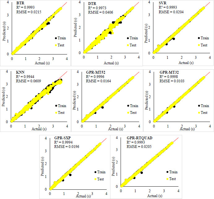
Performance of ML models in predicting the Fundamental Period (FP).
6.2. Distribution of Residuals
In this section, the analysis focuses on the distribution of residuals obtained for the different models, using both the training and testing datasets. Figure 5 illustrates the corresponding distributions. The DTR and KNN models are characterised by the widest residual distributions for both the training and test sets. They also exhibit relatively high standard deviations, indicating greater dispersion of errors and, consequently, a more limited generalisation capability compared to the other models. In contrast, the GPR models display narrower and more symmetric distributions centred around zero, reflecting smaller and more stable residuals overall. This behaviour is particularly evident for the GPR-MT32 model, whose distribution appears the most compact and well-centred.
Furthermore, the mean residuals remain close to zero across all models, suggesting the absence of systematic bias in the predictions. Regarding the distribution shape, the presence of extreme values is observed across all models, as indicated by the high kurtosis values—typical of leptokurtic distributions—both in the training and test data. Finally, the skewness values are negative in the training data for all models, indicating a slight leftward asymmetry, while they become positive for the GPR and SVR models in the test data, denoting a right-skewed distribution.
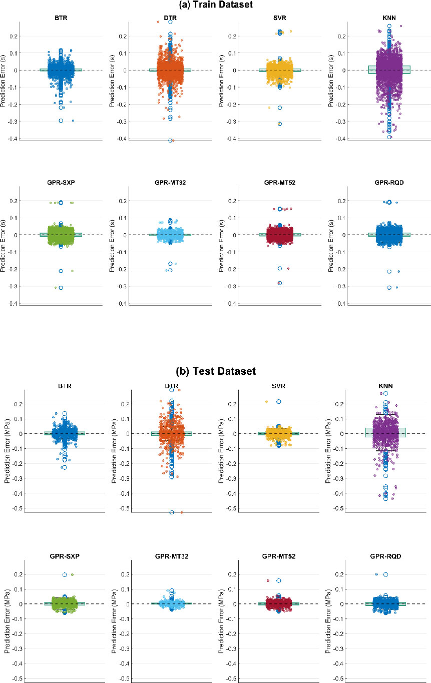
Error distribution for the ML models.
6.3. Taylor Diagram Analysis
The Taylor diagram, proposed by the geophysicist Taylor [52], is a graphical tool widely used in the scientific literature to compare the performance of machine learning models [53-55]. It provides a concise and comprehensive evaluation of model performance based on three key metrics: the correlation coefficient, the standard deviation, and the centred Root Mean Square Deviation (centred RMSD).
The results of this analysis are presented in Fig. (6). It appears that all models exhibit correlation coefficients greater than 0.99 in both the training and test datasets. The GPR models stand out with the highest correlation values across both sets, showing slightly better performance on the test data, demonstrating strong generalisation capability. Moreover, for all models, the standard deviations obtained for the training and testing datasets are close to the reference values, indicating that the variability of the observations is accurately reproduced, with no noticeable tendency toward overestimation or underestimation. A very low centred Root Mean Square Deviation (RMSD) is also observed for both datasets, particularly for the GPR models, confirming their high accuracy and stability. In contrast, the KNN and DTR models exhibit the highest RMSD values for both the training and testing datasets. The increase observed in the testing set reflects a lower generalisation capability, as illustrated in Fig. (6), where these models appear furthest from the reference line.
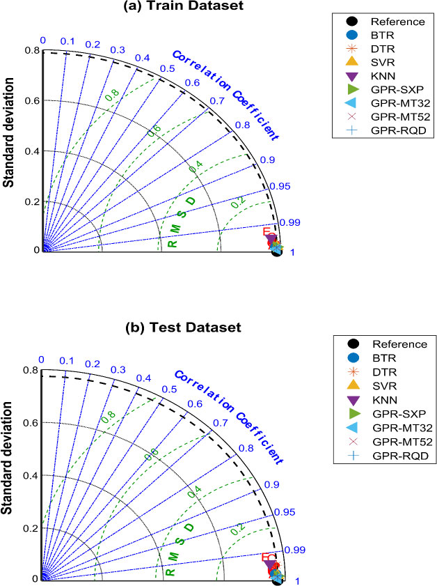
Taylor diagram for training and testing data.
7. COMPARISON WITH PREVIOUS STUDIES
A comparative evaluation was conducted between the GPR-MT32 model developed in the present study and several machine learning models reported in the scientific literature (Table 7). This comparison is based on the values of the coefficient of determination (R2) and the Root Mean Square Error (RMSE) obtained on the test data. Most recent studies rely on the Asteris Database [21], which is also used in this work. Among the most commonly employed algorithms are Random Forest Regression (RFR), Gradient Boosted Tree Regression (GBTR), XGBoost, and Support Vector Regression (SVR).
The comparative analysis highlights the strong competitiveness of the GPR-MT32 model, demonstrating the relevance of Gaussian Process Regression for predicting the fundamental period of Reinforced Concrete (RC) frames infilled with masonry. The model ranks among the best-performing approaches, achieving an R2 = 0.9999 and an RMSE = 0.0091, values that surpass those of most models reported in the literature. However, it is slightly outperformed by the model of Yahiaoui et al. (2025) [28] (R2 = 0.9999; RMSE = 0.0081).
The performance of the GPR-MT32 model is closely followed by that of Shan Lin et al. (2025) [25] and Rahman et al. (2024) [29], who reported R2 = 0.9998 and RMSE values ranging between 0.0113 and 0.0126. These models exhibit performance significantly superior to that of conventional Artificial Neural Networks (ANNs) — for instance, Đorđević & Marinković (2024) [26] reported RMSE = 0.0260, and Mirrashid & Naderpour (2022) [56] reported RMSE = 0.0257. The DTR model reported by Dauji (2024) [30] shows performance comparable to that observed in this study, with a coefficient R2 > 0.99. In contrast, the model proposed by Joshi et al. (2014) [57] yielded the least satisfactory results, which can be explained, at least in part, by the inadequate adaptation of the algorithm to the dataset.
| Reference | ML Algorithms | Dataset | R2 | RMSE |
|---|---|---|---|---|
| Asteris & Nikoo (2019) [20] | ABC-NN | 4026 | 0.9990 | 0.0239 |
| Bioud et al. (2023) [34] | Deep Neural Network (DNN) | 4026 | 0.9997 | 0.0130 |
| Dauji (2024) [30] | DTR | 4026 | 0.9988 | 0.0273 |
| Đorđević & Marinković (2024) [26] | ANN | 2178 | 0.9992 | 0.0260 |
| Inqiad et al. (2024) [33] | XGBoost – GEP - MEP | 569 | 0.9960 | 0.0125 |
| Joshi et al. (2014) [57] | Genetic Programming | 206 | 0.9801 | 0.0100 |
| Karampinis et al. (2024) [24] | GBTR | 4026 | 0.9932 | 0.0723 |
| Kumar et al. (2025) [36] | ANN, RFR, SVR, GBTR | 162 | 0.9995 | 0.0170 |
| Latif et al. (2022) [32] | XGBoost, DNN | 4026 | 0.9966 | 0.0535 |
| Mirrashi & Naderpour [56] | ANN - ANFIS | 4026 | 0.9995 | 0.0257 |
| Rahman et al. (2024) [29] | LightGBM – XGBoost – GBTR - DTR – RFR – CatBoost - NGBoost | 4026 | 0.9998 | 0.0126 |
| Shan Lin et al. (2025) [25] | Kolmogorov-Arnold Network, SVR, CatBoost, XGBoost, RFR, | 4026 | 0.9998 | 0.0114 |
| Somala et al. (2021) [43] | XGBoost – RFR- DTR –LR-SVR-KNN-AdaBoost- Ridge regression | 4026 | 0.9990 | 0.0180 |
| Thisovithan et al. (2023) [31] | ANN, SVR, KNN, RFR | 4026 | 0.9890 | 0.0820 |
| Vijayan et al. (2024) [23] | RFR, LR, SVR, Ensemble Regression | 4026 | 0.9892 | 0.0830 |
| Yahiaoui et al. (2023) [27] | GBTR, lighGBM, CatBoost | 4026 | 0.9998 | 0.0113 |
| Yahiaoui et al. (2025) [28] | RFR, XGBoost, DNN | 4026 | 0.9999 | 0.0081 |
| This study | GPR-MT32 | 4026 | 0.9999 | 0.0091 |
8. SENSITIVITY ANALYSIS
8.1. SHAP-based Sensitivity Analysis
Machine Learning (ML) models are often regarded as “black boxes”, which limits the interpretability of their predictions. To address this issue, several interpretability techniques have been developed, including Partial Dependence Plots (PDP), Individual Conditional Expectation (ICE), and SHapley Additive exPlanations (SHAP), which are widely used in the literature [25, 31–33]. SHAP provides a unified framework based on Shapley values from cooperative game theory, originally introduced by Shapley (1997) [58]. It attributes the model prediction to individual input features by computing their marginal contributions across all possible feature combinations.
The SHAP value associated with a feature i represents its average contribution to the prediction over all possible subsets of features and is mathematically defined in Eq. (8) [59]:

Where N denotes the set of all input variables, n their total number, and S a subset of features not containing i. The function υ(S) represents the model prediction based on the subset S, while the term [υ(S ∪ {i}) – υ(S)] corresponds to the marginal contribution of feature i.
The analysis based on SHAP values (Figs. 7 and 8), including interaction terms, highlights that the fundamental period of reinforced concrete frames is mainly governed by the building height (STN), as previously reported in the literature. The number of storeys (STN) exerts a major influence: the slenderness of the structures tends to increase the fundamental period, whereas low-rise structures have the opposite effect. The interaction between height and the percentage of openings (STN*OPP) amplifies this effect, confirming that a combination of a high slenderness ratio and a large proportion of openings (or even the absence of infills) leads to a significant increase in the fundamental period (FP). The interaction between the height of the structure and the stiffness of the infill walls (STN*IFS) underlines the moderating role of the masonry panels: for a given height, increasing the stiffness of the walls reduces the fundamental period, while lower stiffness values lead to an increase. The joint effect between the percentage of openings and the wall stiffness (OPP*IFS) confirms the complex nature of the infill walls: large openings reduce their stiffness, whereas in the absence of openings and with high stiffness, they contribute significantly to reducing the period. Conversely, the span length (SPL) and the number of spans (SPN) exhibit more modest direct effects; their influence becomes significant only through interactions, particularly with the height of the structure, as highlighted by the influence of STN*SPN and STN*SPL. These results confirm the non-linear nature of the height effect and its dependence on the degradation of stiffness induced by the presence of openings.
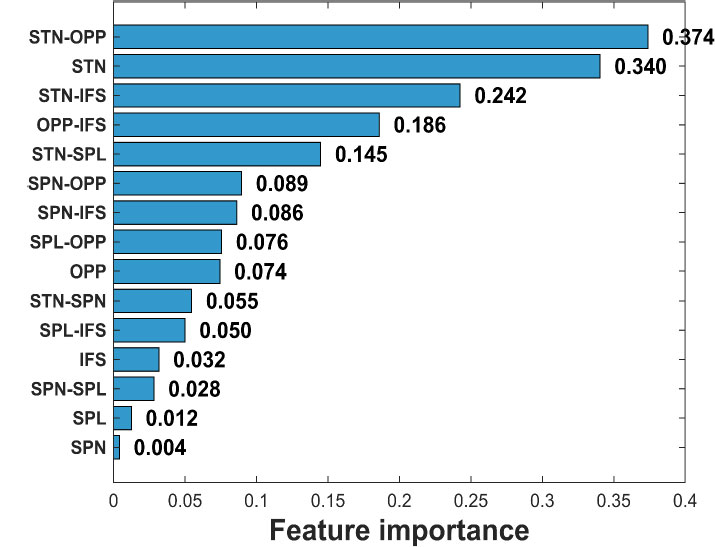
Contribution of the features based on SHAP analysis.
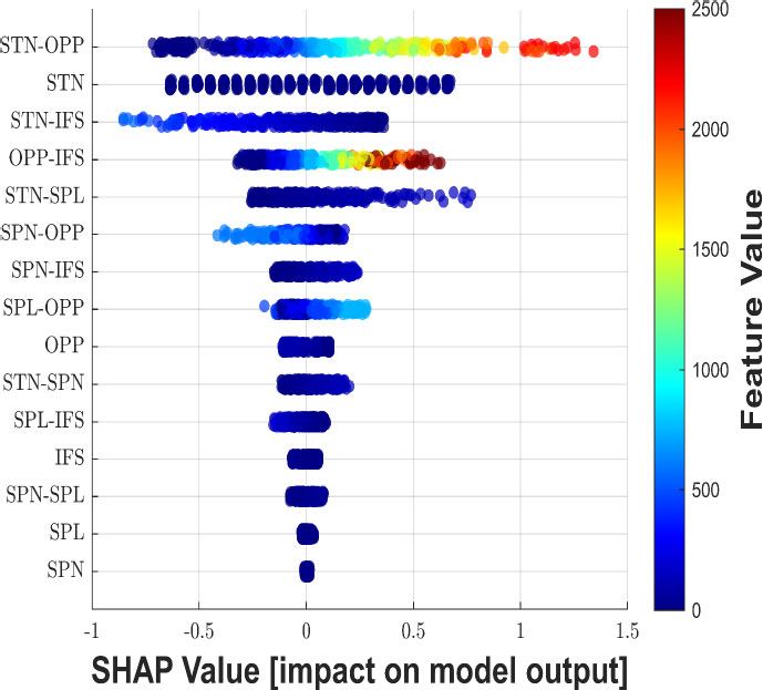
SHAP summary plot.
It should be noted that SHAP values provide a model-based interpretation of feature contributions and reflect the influence of variables within the learned predictive framework. Therefore, the identified effects should be interpreted as indicative of variable importance and interaction patterns rather than strict causal relationships.
Furthermore, the results presented here align with global trends observed across the dataset, while local SHAP values may exhibit variations depending on specific structural configurations.
The findings are consistent with previous studies [26, 31-33]. However, unlike these works, which do not explicitly incorporate interaction variables, the present analysis demonstrates the importance of including them in the study of the dynamic behaviour of reinforced concrete frames.
8.2. Global Uncertainty Propagation Analysis
Uncertainty propagation in a model encompasses all approaches aimed at quantifying how uncertainties present in the input parameters or data are transmitted to the model response. It seeks to estimate the statistical characteristics of the output variable (mean, standard deviation, probability density function, cumulative distribution function, etc.), thereby providing a comprehensive assessment of the model’s reliability. Classical methods include Monte Carlo approaches [60-62] and Polynomial Chaos Expansion (PCE) techniques [63-65]. More recently, Bayesian machine learning approaches, such as Bayesian Neural Networks [66-67], have been developed to probabilistically estimate the model output while explicitly accounting for both epistemic and aleatory uncertainties.
In this section, an uncertainty propagation analysis is performed to quantify the overall variability of the model predictions [48]. The propagation of uncertainty was conducted using the GPR-MT32 model, where the input vector X = [X1, X2,…, Xd] includes both the primary variables and their interaction terms. Consequently, the input variables are not statistically independent, as several components of X are derived from combinations of the basic parameters (e.g., STN*OPP, STN*IFS). These input variables represent structural characteristics related to stiffness, geometry, and infill configuration, and therefore inherently reflect physical sources of variability observed in real structures.
For each sampled input x(i), the GPR model provides a probabilistic prediction in the form of a normal distribution, as expressed in Eq. (9):

μ(x(i)) et σ2(x(i)) denote the predictive mean and variance estimated by the GPR. The uncertainty propagation is then based on a Monte Carlo sampling scheme, in which each realisation of the output variable is generated according to Eq. (10):

From the ensemble of N generated realisations, the statistical descriptors of the model response are empirically estimated. The probability density function (PDF) fY(y) is estimated using the Gaussian Kernel Density Estimation (KDE) method, while the cumulative distribution function (CDF) is computed as shown in Eq. (11):
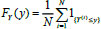
From this empirical distribution, several statistical descriptors are derived, including the expected value μY, the variance Var(Y), the standard deviation, and the empirical quantiles (2.5th and 97.5th percentiles), which define a 95% confidence interval [48]. The number of Monte Carlo simulations was set to 50,000, as convergence tests on the mean and variance indicated variations below 1%, ensuring the stability and reliability of the estimated global uncertainty metrics.
The uncertainty propagation, conducted via Monte Carlo sampling based on the GPR-MT32 model, highlights a pronounced variability in the predicted Fundamental Period (FP). The Probability Density Function (PDF) exhibits a moderately right-skewed distribution (Fig. 9), indicating that most predictions cluster around lower FP values while a smaller fraction extends towards higher ones. The range of relevant realisations spans from -0.343 seconds to 3.448 seconds. The results yield a mean of 1.418 seconds, a standard deviation of 0.970 seconds, and a variance of 0.940 seconds2, corresponding to a coefficient of variation of approximately 68.4%. This high dispersion reflects the strong sensitivity of the fundamental period to variations in the structural parameters governing the mass and stiffness distributions.
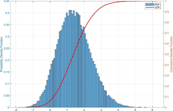
Uncertainty propagation for the optimal model.
The Cumulative Distribution Function (CDF) exhibits a smooth sigmoidal shape, indicating well-behaved and controlled dispersion of the results. The CDF analysis shows that 50% of the simulations produce a period less than 1.374 seconds, 90% lower than 2.692 seconds, and 95% lower than 3.079 seconds. This distribution reflects both the nonlinear dependence of FP on the governing parameters and the influence of uncertainty in poorly sampled regions of the input space.
A variance decomposition was performed to clarify the origin of the overall uncertainty. By applying the law of total variance to the predictive components of the GPR model, a total variance of Var(FP) = 0.940 seconds2 was obtained, of which 7.8% is attributable to model (epistemic) uncertainty and 92.2% to input (aleatory) uncertainty. This result indicates that predictive dispersion is predominantly driven by the variability of structural parameters rather than by intrinsic limitations of the model.
Additionally, a small proportion of negative values (FP < 0) was observed, representing approximately 6.34% of all realisations. These outcomes reveal a limitation of the model, as the fundamental period cannot take negative values. To enhance the physical consistency of the predictions, it would be relevant to employ physics-informed approaches such as the Deep Energy Method (DEM) [68-69] and its extension VINO [70], which explicitly embed physical laws into the learning process.
CONCLUSION
This study focused on predicting the fundamental period of Reinforced Concrete (RC) frames infilled with masonry using Gaussian Process Regression (GPR) models. To this end, an in-depth comparison was carried out among several advanced machine learning models, including Decision Tree Regression (DTR), Support Vector Regression (SVR), Bagging Tree Regression (BTR), k-Nearest Neighbours (KNN), and GPR. All models were optimised through a Bayesian hyperparameter tuning approach and evaluated using the FP4026 Research Database across different training and testing data partitioning scenarios, based on statistical indicators and graphical tools. A sensitivity analysis (SHAP approach) and a global uncertainty analysis were subsequently applied to the optimal model. The main findings of this study can be summarised as follows:
- All tested machine learning models demonstrated high performance, with coefficients of determination R2 > 0.99 for both training and testing datasets. However, the GPR-MT32 model stood out with markedly superior performance compared to the other models.
- The Gaussian Process Regression model, hitherto unexplored in the scientific literature for this type of structure, proved particularly effective in predicting the fundamental period—a result further confirmed through comparison with models reported in previous studies.
- The introduction of interaction variables significantly improved the accuracy of all models, highlighting their importance in capturing nonlinear behaviours.
- The sensitivity analysis conducted using the SHAP method revealed the dominant influence of interaction variables over linear ones, confirming the nonlinear nature of the relationship between the input variables and the fundamental period.
- Among the most influential interactions is that between the number of storeys (STN) and the percentage of openings (OPP), which strongly affects the overall stiffness of the frame: as building height and openings increase, stiffness decreases, leading to a higher fundamental period. The interaction between STN and the infill stiffness (IFS) also shows a significant effect, albeit less pronounced than that of the number of storeys considered alone.
- These findings emphasise the importance of accounting for interaction effects when training machine learning models: some variables that may appear marginal become significant when combined with other structural parameters.
- Finally, the global uncertainty analysis showed that the GPR-MT32 model exhibits variability in its predictions mainly due to input uncertainty (92.2%), with model uncertainty (7.8%) remaining low. This indicates that predictive variability is predominantly driven by variability in structural parameters (e.g., stiffness, mass distribution, and infill configuration) rather than model limitations. However, the presence of a few negative values, although marginal, highlights one of the inherent limitations of purely data-driven approaches.
LIMITATIONS AND FUTURE PERSPECTIVES
This study is based on a purely data-driven approach aimed at analysing the performance of Gaussian Process Regression (GPR) models for predicting the fundamental period of reinforced concrete frames infilled with masonry. Several simplifying assumptions were adopted. The database used represents the behaviour of a single frame, without considering the orthogonal direction; consequently, the influence of floor slabs was neglected. Another simplification concerns the exclusive consideration of frames with uniform distributions of mass and stiffness—a potential direction for future research is to investigate the effects of irregularities in these distributions. Furthermore, the span length was kept constant, unlike in real structures, where spans typically vary from one bay to another.
A further limitation concerns the presence of multicollinearity induced by the inclusion of interaction variables. As these terms are inherently correlated with their parent variables, relatively high Variance Inflation Factor (VIF) values were observed. While this does not affect the predictive performance or stability of the GPR model—owing to its kernel-based formulation and implicit regularisation—it may influence the interpretability of feature attribution methods such as SHAP. Consequently, the interpretation of feature contributions should be approached with caution and primarily considered at a global level. Future work may explore alternative strategies such as feature orthogonalisation or dimensionality reduction to further improve interpretability. Although the impact of interaction terms on predictive performance was not explicitly isolated, the overall results suggest that their inclusion contributes to capturing complex nonlinear relationships.
The present study relies on the Asteris FP4026 database, which is generated from numerical simulations rather than field or experimental data. This dataset is based on simplified planar numerical simulations and may not fully capture the complexity of three-dimensional structural behaviour. Consequently, the learned relationships reflect the modelling assumptions embedded in the simulation framework, including material behaviour, boundary conditions, and infill–frame interaction. In addition, the set of input variables is limited and may not capture all parameters influencing the fundamental period of infilled frame structures. The validity of the results is further restricted to the range covered by the database, and the proposed models should therefore be interpreted as representative of the simulated domain; caution is required when extrapolating findings to actual buildings.
This research has also highlighted one inherent limitation of purely data-driven approaches, in which the model is not constrained by physical laws. In this regard, the integration of physics-informed methods represents a particularly promising avenue for future investigation. More broadly, future work should consider more comprehensive datasets incorporating three-dimensional modelling, additional relevant variables, and experimental or field data to further validate and enhance the robustness and external validity of the approach.
AUTHORS’ CONTRIBUTIONS
The authors confirm contribution to the paper as follows: M.A., K.B.;: Conceptualization; M.A., K.B. Methodology; M.A., K.B.: Software; M.A., B.M.: Validation; M.A.: Formal analysis; M.A., B.M.: Investigation; M.A.: Data curation; M.A.: Visualization; M.A.: Writing—original draft preparation; M.A., K.B., B.M.: Writing—review and editing; K.B., B.M.: Supervision. All authors have read and agreed to the published version of the manuscript.
LIST OF ABBREVIATIONS
| A20 index | = Ratio of tests for which the prediction is within ± 20% of the experimental value across the entire dataset |
| A30 index | = Ratio of tests for which the prediction is within ± 30% of the experimental value across the entire dataset |
| BTR | = Bagging Tree Regression Model |
| COV | = Coefficient of Variation |
| DTR | = Decision Tree Regression Model |
| FP | = Fundamental Period |
| GPR-MT32 | = Gaussian Process Regression model with Matern 3/2 Kernel |
| GPR-MT52 | = Gaussian Process Regression model with Matern 5/2 Kernel |
| GPR-SXP | = Gaussian Process Regression model with Squared Exponential Kernel |
| GPR-RQD | = Gaussian Process Regression model with Rational Quadratic Kernel |
| IFS | = Infill Stiffness |
| KNN | = K-Nearest Neighbours |
| MAE | = Mean Absolute Error |
| MAPE | = Mean Absolute Percentage Error |
| OPP | = Percentage of opening in the masonry infill wall. |
| R2 | = Coefficient of Determination |
| RFR | = Random Forest Regression |
| RMSE | = Root Mean Square Error |
| SHAP | = SHapley Additive exPlanations. |
| SVR | = Support Vector Regression model |
| STN | = Storey Number |
| SPL | = Span Length |
| SPN | = Span Number |
AVAILABILITY OF DATA AND MATERIALS
All the data and supporting information are provided within the article.
ACKNOWLEDGEMENTS
Declared none.